Lora localization in Jupyter
This post shows a localization visualization in Jupyter that uses LoraWan receptions of TheThingsNetwork to localize
Introduction
In my previous post I presented a cheap and simple LoraWan node:
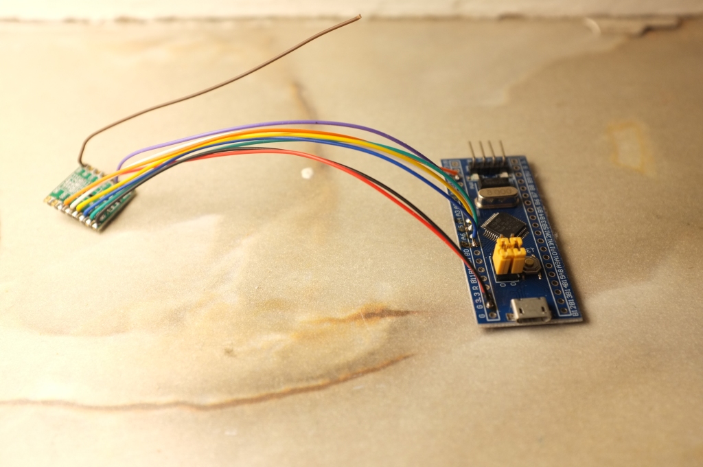
There are of course many things you could do with such a device: Home automation, weather stations, etc. In this post we will however take a closer look at a tracking application. In this type of application you typically want to know the location of “something” and communicate this information. Communication is in this context quite clear (Lora), but what about localization?
The first thing that comes in mind is of course GPS. The receivers are cheap, easy to integrate and deliver quite good global localization in the meter range accuracy. But… these devices typically only work if you are having a clear line of sight to the satellites. In most cases this means that you need to be outdoors to use them. What to do if your project requires indoor usage? Or underground usage, where you even won’t have any Wifi signals which you could use for localization?
This page presents an alternative to GPS that uses the receive signal strength (RSSI) of Lora receptions to estimate the position of the transmitter. The accuracy that one can expect from such a solution is of course orders of magnitude lower than GPS. But in theory this should also work indoors and (relatively) deep underground.
TheThingsNetwork data
Whenever a node sends a packet in TheThingsNetwork, you not only get the data of the node but also some very helpful metadata. Here you can see an example of the data you get:
OrderedDict([('app_id', 'befinitiv-testnode'),
             ('dev_id', 'testnode'),
             ('hardware_serial', '009B45E4337B4515'),
             ('port', 1),
             ('counter', 49),
             ('payload_raw', '9gEcAQ=='),
             ('metadata',
              OrderedDict([('time', '2020-04-01T07:06:54.901217967Z'),
                           ('frequency', 868.3),
                           ('modulation', 'LORA'),
                           ('data_rate', 'SF10BW125'),
                           ('airtime', 329728000),
                           ('coding_rate', '4/5'),
                           ('gateways',
                            [OrderedDict([('gtw_id', 'eui-fcc23dfffe0e316a'),
                                          ('timestamp', 721532820),
                                          ('time', ''),
                                          ('channel', 1),
                                          ('rssi', -103),
                                          ('snr', 2.5),
                                          ('rf_chain', 0)]),
                             OrderedDict([('gtw_id', 'eui-60c5a8fffe76636c'),
                                          ('timestamp', 2549255116),
                                          ('time', ''),
                                          ('channel', 6),
                                          ('rssi', -82),
                                          ('snr', 5.5),
                                          ('rf_chain', 0)])])]))])
As you can see above, TTN tells us that our node was seen by two gateways with the IDs “eui-fcc23dfffe0e316a” and “eui-60c5a8fffe76636c”. It also tells us the receive signal strength (RSSI) of -103 and -82dBi respectively. The only other ingredient you need is to know the location of the gateways to estimate the location of your node. Luckily, TTN lets you query this information:
https://www.thethingsnetwork.org/gateway-data/gateway/eui-fcc23dfffe0e316a
With all this info at hand, you should be able to guesstimate the location of your node. But there are still many unanswered questions: How many gateways typically receive data from your node, how stable and meaningful are the RSSI values, …? To answer these questions I developed a visualization of the data that will be presented in the next section.
Jupyter map visualization of TTN data
As said above, even though the theory of RSSI localization is simple, there are still many questions to answer. And the best way in this case to find answers is to visualize the data that we receive.
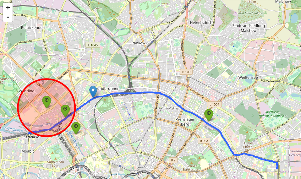
Therefore, I developed a Jupyter notebook that visualizes the data as follows:

The image above shows gateway position with green markers, receptions from the node as red circles which are scaled by the RSSI value and the position of the node as a blue marker. The position of the node has been determined by GPS to have a reference to better understand the TTN measurements. The GPS track is also shown as a blue line on the map.
The notebook works in two modes:
- Live
- Replay
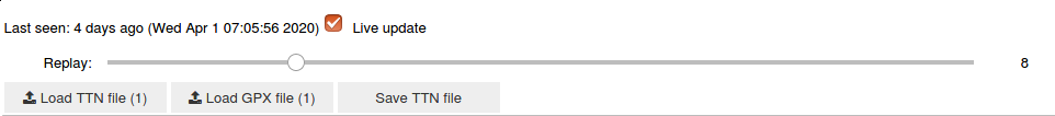
In live mode, the notebook connects to TTN and immediately displays receptions of your node on the map. These receptions can also be stored in a file for later analysis. If you load this file, you can use the replay mode to scroll through all the receptions of your node over time. To have some kind of reference measurement, you can also load a GPX file into the map. GPX position and TTN data are then associated via their timestamps. The following image shows the gui elements of the notebook:
Usage of the notebook
Thanks to the MyBinder service, you can use the notebook simply by clicking on the following link: https://mybinder.org/v2/gh/befinitiv/ttn_map_localization/master?filepath=ttn_map_localization.ipynb
(Note that MyBinder does not allow network connections, so live connection to TTN is not possible)
To run the notebook on your machine, all you need to do is:
git clone https://github.com/befinitiv/ttn_map_localization.git
pip3 install jupyter-repo2docker
jupyter-repo2docker -E ttn_map_localization
The repository contains an example TTN recording of my node of a drive through Berlin as well as the GPX file of that drive.
Analysis of the data
As said before, the purpose of the notebook is to get a feeling of the data. I will now share my impressions of the data and how suitable I find it for the purpose of localization. Please note that the data I am talking about is also included in the repository as the example files (.tickle and .gpx) so you as well can get first hand experience of the data.
Stability
The easiest way to assess stability is to look at a time where the node is not moving:

The picture above looks quite reasonable. All but one gateway received data and also the RSSI readings seem quite reasonable. However, without the node moving, just 20s later the data looks like this:

In the image above, only one gateway received a signal, and this time also a much stronger signal. Mmmh, stability-wise not great. And you find many other such examples in the data.
Completeness
The node was sending packets every 20s. The question of completeness is: How many of these packets were received by TTN? And the answer to this is unfortunately: Not that many. In fact, there are quite significant gaps in the data, in the order of several kilometers without any reception.
For example, from here:
to here:

we received nothing at all. The drive was done using a train that runs above ground. Granted, the tracks on this section are in a trench but still, no reception at all is quite disappointing.
Sensibility
The following image shows an example that makes me question whether I or TTN have a bug somewhere:
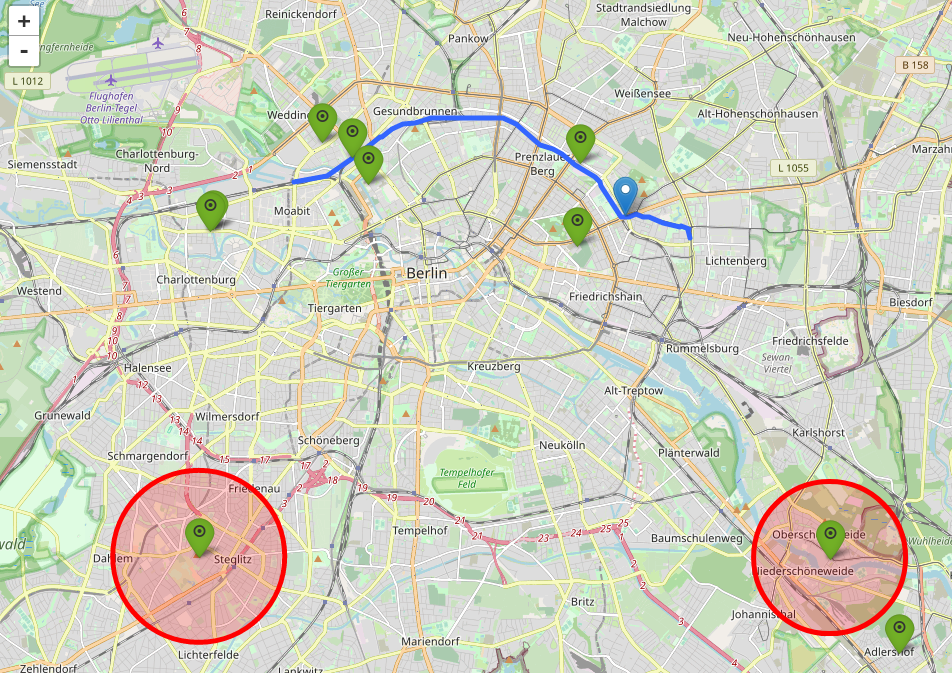
The problem with the image above: Why don’t the closest gateways to our node receive the data but instead gateways very far away? Especially the “Steglitz” gateway is _really_ far off. The distance between the node and gateway is 13km, crossing through the inner city of Berlin. This seems to me quite unlikely, especially in combination with the close-by gateways receiving nothing.
Another odd example is shown in the following image:

Above you see a gateway at 8km distance showing an RSSI comparable to the node being right next to the same gateway:

Conclusion
In summary, the data that I received from TTN seems a bit odd to me. Of course I could imagine explanations for all the odd cases I encountered but to my eye the data just does not look 100% right. This might be due to a bug hidden in my code or TTN or (and more likely) due to my lack of experience with Lora signal propagation in urban environments.
I never had the expectation of getting close to the 1m accuracy of GPS, not even 10m. My hopes were more in the range of a couple of 100m. But after looking at the data, I am more inclined to say that such a localization could just tell me “Berlin” or “not Berlin”, which is of course in many cases not really helpful.
I would highly appreciate if someone experienced with Lora signal propagation could shed some light into the oddities I found in the comment section.
